FROM SCORES TO SAMPLES

Elastic Forcing.

From Scores to Samples: Elastic Forcing
for Autoregressive Video Generation

Chi Zhang1,*Yueyi Liu1,2,*Haoyang Shi1,3,*Ruichuan An4Haoyu Li2Yuhang Wu1Sen Cui5Miao Liu1,†
1College of AI, Tsinghua University2IAIR, Xi’an Jiaotong University3Xianghui Academy, Fudan University4Peking University5BAAI

* Equal contribution · † Corresponding author

01 / THE CORE IDEA

Learn from samples.
Leave the score models behind.

Elastic Forcing post-trains few-step autoregressive video generators directly against reference videos. Frozen video representations make the two distributions comparable; maximum mean discrepancy (MMD) supplies the training signal.

THE BOTTLENECK

Score-based post-training carries extra models.

Distribution Matching Distillation uses a diffusion teacher and an online fake-score model alongside the generator. Those auxiliary models add memory and computation, and the teacher defines the supervision.

OUR ALTERNATIVE

The reference collection defines the target.

Match generated and reference video features directly. Only the generator is optimized during post-training; feature encoders and precomputed reference statistics stay frozen.

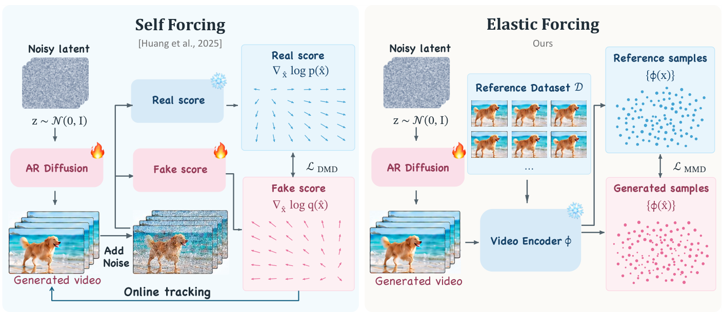
Self Forcing uses real and fake score models; Elastic Forcing instead compares generated video features with reference video features through MMD.
From score matching to sample matching. The autoregressive rollout is retained while score-based supervision is replaced by direct distribution matching. Figure 2 in the paper ↗

This change applies to distributional post-training. The standard experiments still start from pretrained, ODE-initialized checkpoints; it is not a claim of training from scratch without a pretrained model.

02 / HOW IT WORKS

Better estimates.
A smaller backward pass.

Reliable distribution matching needs many video samples. Elastic Forcing separates the statistics needed to estimate the loss from the computation needed to differentiate it.

01 / REPRESENTATION SPACE

Compare what happens,
not just pixels.

V-JEPA 2 captures predictive temporal features. VideoMAE adds spatiotemporal structure. The three-encoder variant also uses DINOv3 for frame-level semantics.

MMD compares the generated and reference distributions within each frozen feature space. The reference–reference term is constant with respect to the generator.

Objective · Section 3.1 ↗
V-JEPA 2VideoMAE+ DINOv3
Generated features
Reference features
LEF = Σe λe MMD²(Pθe, Prefe)

Generated–generated interactions + generated–reference interactions

02 / THE REFERENCE SIDE

A stable summary.
A fresh correction.

A persistent Nyström summary incorporates the full reference collection without comparing every query against every video. Its finite rank can introduce approximation bias.

Monte Carlo estimates from sampled references are unbiased but noisy. Blending the two balances approximation bias and sampling variance.

Hybrid estimator · Section 3.2 ↗
PRECOMPUTEDNyström summaryPersistent, full-collection statistics
SAMPLED EACH UPDATEMonte Carlo referencesFresh minibatch estimates
m̂ref(z) = (1 − α)mNys(z) + αm̂MC(z)

One hybrid reference estimate · Equation 9

03 / THE GENERATED SIDE

Estimate with more.
Backpropagate through fewer.

Evaluate the MMD interactions across a large population of fresh rollouts in feature space. Then replay a uniformly sampled subset to propagate the feature gradients through the generator.

Rescaling by B/b gives a conditionally unbiased estimate of the evaluated full-batch gradient. Sparse boundary states make replay practical without retaining every rollout graph.

Selective differentiation · Section 3.3 ↗
256rollouts for distribution estimation
B · default 1.3B setup
Full-population feature interactionsUniform subset + local replay
128rollouts for backpropagation
b · default 1.3B setup

Only the generator is updated.

03 / RESULTS

Stronger generation.
Room to scale.

84.64

VBench Total

1.3B, two encoders
vs. 83.80 for Self-Forcing

17 FPS

Same inference throughput

1.3B comparison
as reported in Table 1

14B

Post-trained on 8 H200 GPUs

80 updates · 23.2 hours
5 denoising steps per chunk

1.3B autoregressive generation · VBench (Table 1)
MethodTotal ↑Quality ↑Semantic ↑FPS ↑
CausVid82.8883.9378.6917.0
Self-Forcing83.8084.5980.6417.0
Elastic Forcing 3 encoders84.2585.0680.9917.0
Elastic Forcing 2 encoders84.6485.4381.4817.0

The Elastic Forcing / Self-Forcing comparison uses matched architecture and ODE initialization. Evaluation uses expanded versions of 946 VBench prompts, with five seeds per prompt. Two encoders: V-JEPA 2 + VideoMAE; three encoders: additionally DINOv3. Table 1 and evaluation details ↗

Scaling without auxiliary score networks.

Removing the diffusion teacher and fake-score model makes 14B post-training possible on a single node of eight H200 GPUs. Different offloading strategies trade GPU-hours against peak memory.

In the paper’s 14B comparison, Elastic Forcing achieves a VLM Total score of 4.217 versus 4.115 for Krea Realtime. The 42-participant human evaluation reports mean ratings of 3.354 and 3.054, respectively.

Human results are average ratings, not preference percentages. The 14B experiment uses Krea’s initialization and is separate from the 1.3B VBench comparison.
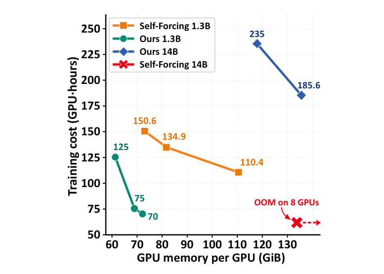
Training cost against peak GPU memory for Self Forcing and Elastic Forcing at 1.3B and 14B scales. Self Forcing 14B is out of memory on eight GPUs.
Training efficiency · Figure 6 ↗

04 / BEYOND THE TEACHER

New references.
New possibilities.

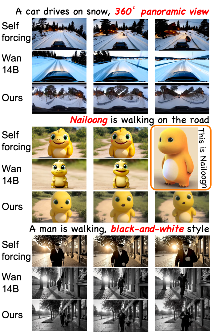
Change the reference videos to change what the generator learns—without first adapting a target-specific diffusion teacher.

01

Spatial priors

Wide-angle references encourage panoramic composition.

02

Character identity

Character-specific videos teach the appearance of Nailoong.

03

Visual style

Black-and-white references lead to monochrome generations.

Reference-data adaptation · Section 5.2 ↗
Figure 7 compares panoramic composition, Nailoong identity, and monochrome style learned from reference videos.
Reference-defined adaptation with the 1.3B generator. Figure 7 from the paper.

05 / THE VIDEO COLLECTION

See it in motion.

Characters. Worlds. Motion.
21 video examples.

A playful character

01

Elastic Forcing

02

Under the ocean

03

Volcanic dusk

04

A field of sunflowers

05

A clash above the clouds

06

Mountains in the mist

07

Waves and volcanic shores

08

Liquid light

09

At the waterfall

10

The blue samurai

11

Under a full moon

12

A view of Earth

13

Through the canyon

14

Islands in the sky

15

In the bamboo forest

16

Across the river

17

A mountain sanctuary

18

Above the clouds

19

The lone swordsman

20

Running above the clouds

21

READ THE PAPER

From Scores to Samples.

Elastic Forcing for Autoregressive Video Generation